The Traveling Salesman Problem (TSP) For Adventurous Types


It's a deceptively complex mathematical conundrum. You have 5, 10, or 20 destinations you want to batch together into a road trip. You need to find the fastest and/or most efficient - i.e. optimal - between them, geographically-speaking.
Our brains work so fast, so effectively, we barely notice the actual difficulty in computing a result. One which we may never find the absolute answer to.
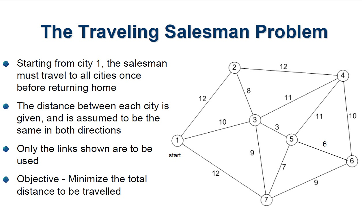
It's what's known in data science terms as the Traveling Salesman Problem, studied in the 1930s, and most simply defined as:
A salesman must travel between N cities. The order in which he does so is something he does not care about, as long as he visits each once during his trip, and finishes where he was at first.
Or, in academic-speak:
"Given a finite number of "cities" along with the cost of travel between each pair of them, find the cheapest way of visiting all the cities and returning to your starting point."
Best Guess: Heuristics & Meta-Heuristics
Broadly-speaking, the TSP is one of many different variants of the Shortest Path Problem, and has a rich history which has captivated mathematicians for a long, long time. It's so complex, it's unlikely to ever be solved acceptably or in an absolute way.
As an example of a PvsNP problem, the issue is one of polynomial time and being NP-complete. In ordinary terms, it means you means you need to be able to solve it properly in a reasonable amount of time - not the time it takes for the universe to end. All of these types of maths problems aim to optimise a process.
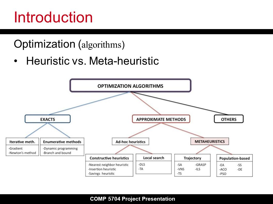
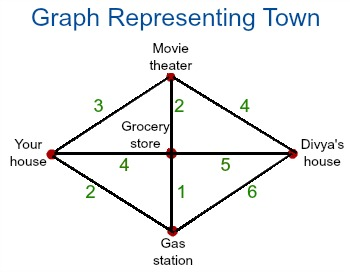
When we can't solve a problem absolutely, but need the best solution we can come up with, we use a heuristic. What's a heuristic?
"Any approach to problem solving or self-discovery that employs a practical method, not guaranteed to be optimal, perfect, or rational, but instead sufficient for reaching an immediate goal. Where finding an optimal solution is impossible or impractical, heuristic methods can be used to speed up the process of finding a satisfactory solution."
The process of attempting to find one, involving the concept of a meta-heuristic. What's one of those?
"A higher-level procedure or heuristic designed to find, generate, or select a heuristic (partial search algorithm) that may provide a sufficiently good solution to an optimization problem, especially with incomplete or imperfect information or limited computation capacity."
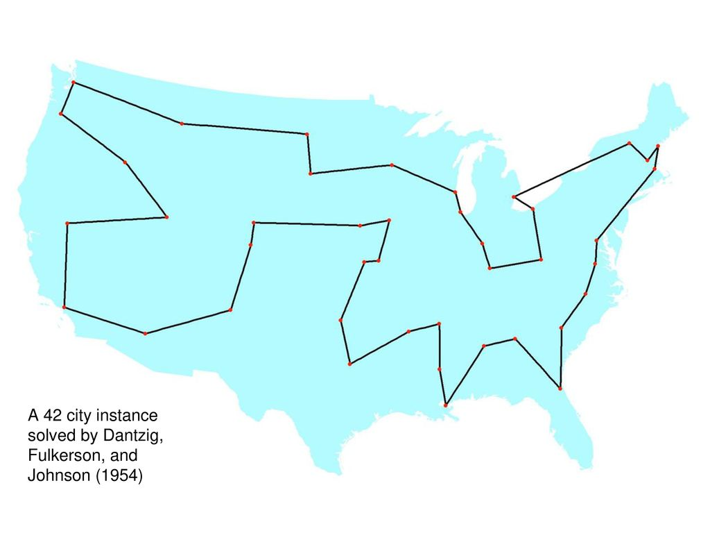
Model Prototype A: Traveling All Contiguous US States
The most extensively debated invocation of said problem, in contemporary terms, is the best way to travel to each of the 48 contiguous US states (excluding Alaska and Hawaii). It could be Europe, or any other continent; it just happens, despite being a British problem, it's been best-studied in North America.
It was formulated as a computer science problem by Dantzig, Fulkerson and Johnson in 1954.
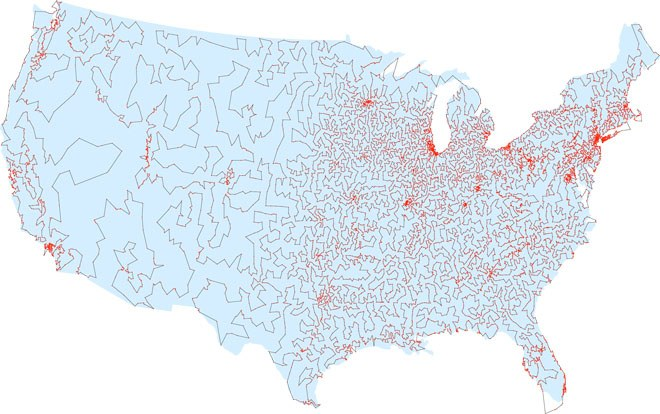
For anyone researching the problem-set, one of the best resources is hosted by the University of Waterloo (Canada), who published their methodology using US geological data which defines 115,475 towns and cities in the United States. They even published a leader board of challengers who attempted the best calculation.
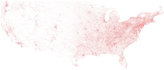
According to Waterloo, a walk across all 49,603 sites would be 217,605 miles:
Iteration: Dijkstra's Shortest Path
In 1956, Edsger W. Dijkstra came up with his solution to the Shortest Path problem, as the field had started to form the domain of Graph Theory.
In academic's terms:
"Dijkstra's algorithm computes the cost of the shortest paths from a given starting node to all other nodes in the graph. The algorithm starts at its starting node and iteratively updates the current shortest paths via the current node. The algorithm may, in the process, find shortcuts. It continues until all edges have been visited and no improvement is possible. The algorithm keeps the nodes that it has found, but not processed yet, in a priority queue. The nodes with the smallest distance to the starting point is the first node in the queue."
Iteration: Commercial Libraries
The TSP has also been studied as a problem by IT companies like SAS, which in this example uses a simplistic SQL methodology (OPTNET) to attempt to list all the possible routes - which, as we will soon discover, is a rather foolish idea:
/* Create a list of all the possible pairs of cities */
proc sql;
   create table CitiesDist as
   select
      a.city as city1, a.lat as lat1, a.long as long1,
      b.city as city2, b.lat as lat2, b.long as long2,
      geodist(lat1, long1, lat2, long2, 'DM') as distance
      from Cities as a, Cities as b
      where a.city < b.city;
quit;
SAS' eventual map of the optimal route across US cities with a total distance of 10,627.75.
Amongst the many large-scale computation networks currently available, systems like Gurobi are the loudest to challenge it on a corporate level. The platform's solution also comes in similar:
Iteration: Karp's Paper & Christofides' Idea
in 1972, computer scientist Richard Karp, of the University of California at Berkeley, declared the problem to be NP-Hard. Four years later jn 1976, Nicos Christofides, a professor at Imperial College London, developed an algorithm which produced routes 50% longer than the promised shortest route.
Christofides' algo starts by looking not for the shortest round-trip route, but the shortest spanning tree — a collection of branches linking the cities, with no closed loops. Unlike the shortest round-trip route, the shortest spanning tree is easy to construct efficiently: Start by finding the shortest highway connecting two cities; that’s the first branch. To add the next branch, find the shortest highway connecting a new city to one of those two — and so on until all the cities have been reached.
40 years later, researchers at McGill produced a route 30% over the anticipated absolute answer (as above).
Iteration: Lin-Kernighan
In 1998, the most famous software suite for solving the problem, the Concorde TSP Solver, was first described in the paper "On the solution of traveling salesman problems", Proceedings of the International Congress of Mathematicians, Vol. III (Berlin, 1998). It was incorporated into an online server version for anyone to use.

The software uses the Chained Lin–Kernighan heuristic, which is based on the graph-partitioning Lin-Kernighan algorithm and described, in near-human-speak, as follows:
"At the beginning it randomly partitions graph on two sets, then it tries to find pair of vertices, one from each set, so as we exchange them, the total number of connections (edges) between those sets decreases."
According the spiel, the TSP solver implements "Delaunay Triangulation, Minimum Spanning Tree, and various Nearest Neighbor Set generators."
Needless to say, the TSP solver "includes over 700 functions permitting users to create specialized codes for TSP-like problems" and "has been used to obtain the optimal solutions to all 110 of the TSPLIB instances; the largest having 85,900 cities".
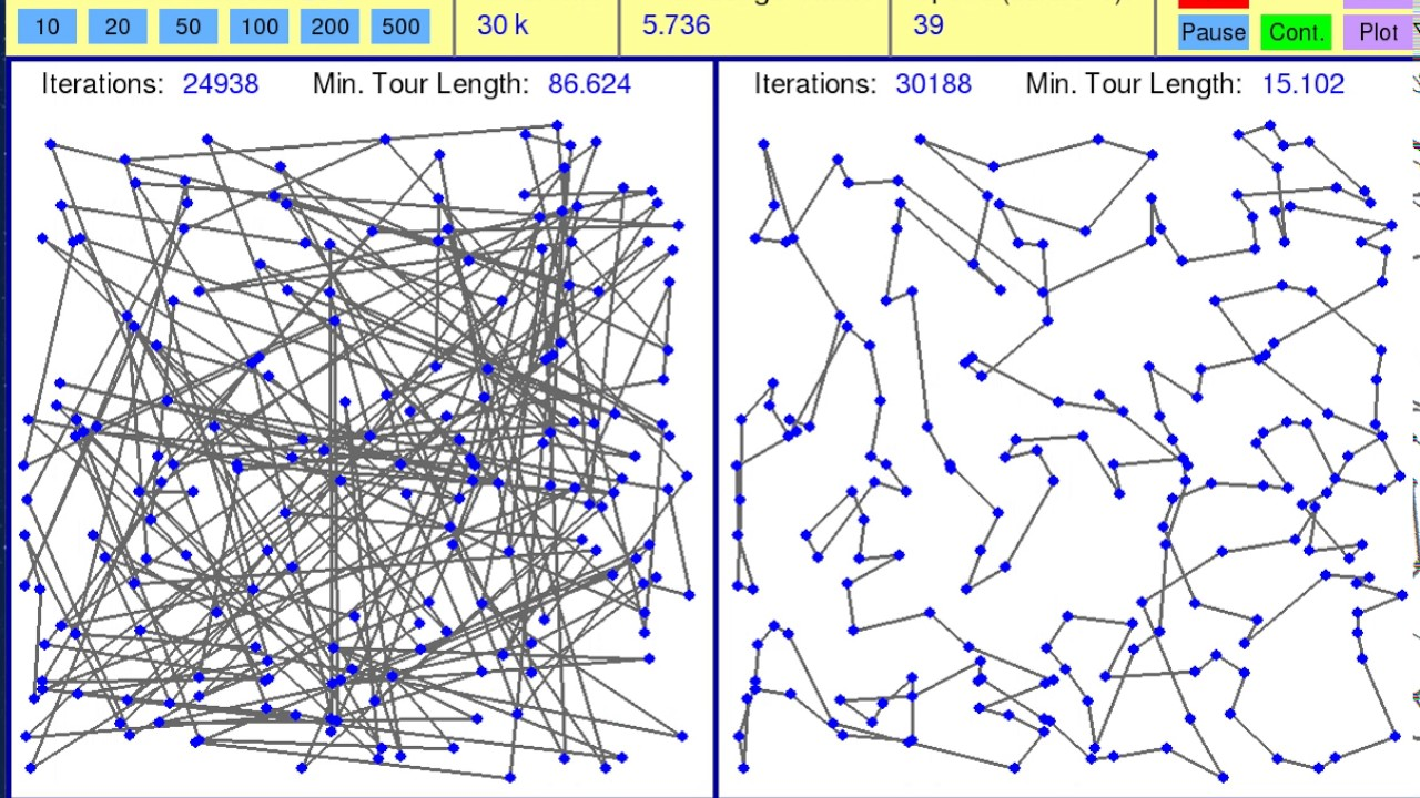
Iteration: Simulated Annealing
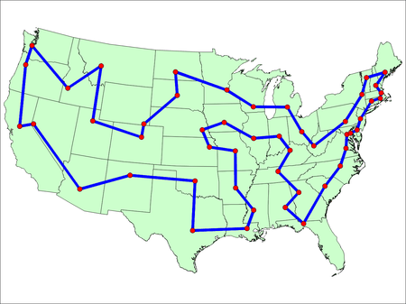
In 2014, a more sophisticated approach was taken by an employee at music data company Genius.com named Todd Schneider, who used a probability technique named Simulated Annealing and published his results on his blog.
A friendly explanation given during commentary:
"Usually, the algorithm starts with a random solution to the problem. Then, that solution is randomly modified, or 'tweaked'. The algorithm then compares the first solution to the second based on their 'fitness'. The fitness is a value which describes how well the solution solves the problem. In this instance, a solution which requires less travel would be considered to be of higher fitness than one which requires more. Normally, the algorithm then chooses the solution which has the best fitness. The interesting thing about Simulated Annealing however, is that it has a chance to pick the worse solution. This allows solutions which previously would not have been seen to now be produced by modifying the new, worse solution. The chance that the algorithm will chose the worse solution is called the temperature, which is controlled by the schedule, seen in the 'Annealing Schedule' graph.. As time goes on, the temperature lessens and decreases the chance of a worse solution being picked. Over time, this creates a convergence of sorts upon ideally the best solution."
The eventual solution:
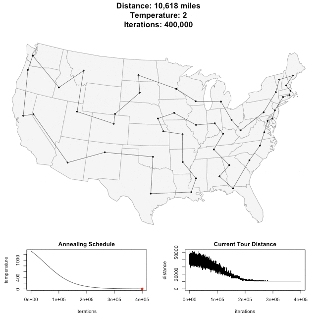
To give an idea of cost: at 25 miles per gallon car at a price of $3.45 requiring 424.72 gallons to travel, the cost of per state would approximate $1,465.
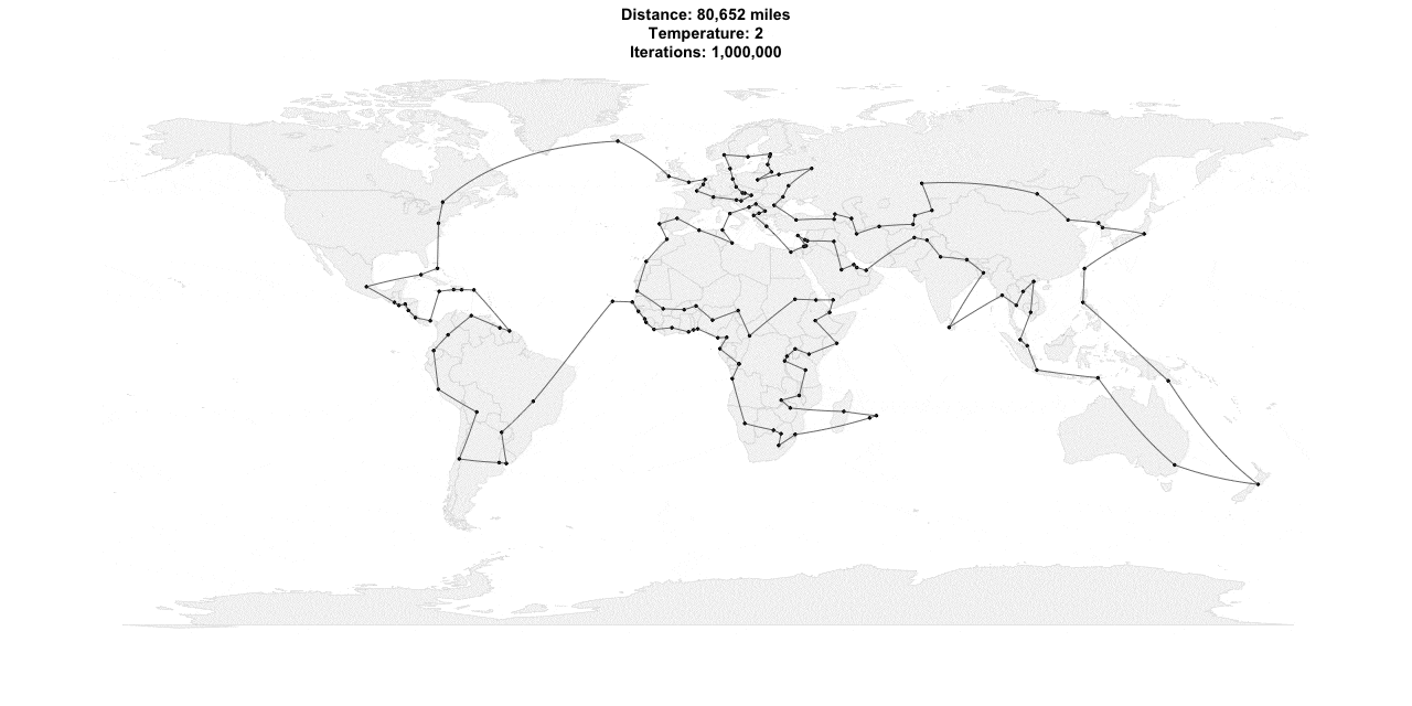
He even applied the same process to all world capital cities, and this was the output at 80,852 miles:
Iteration: Darwin Edition
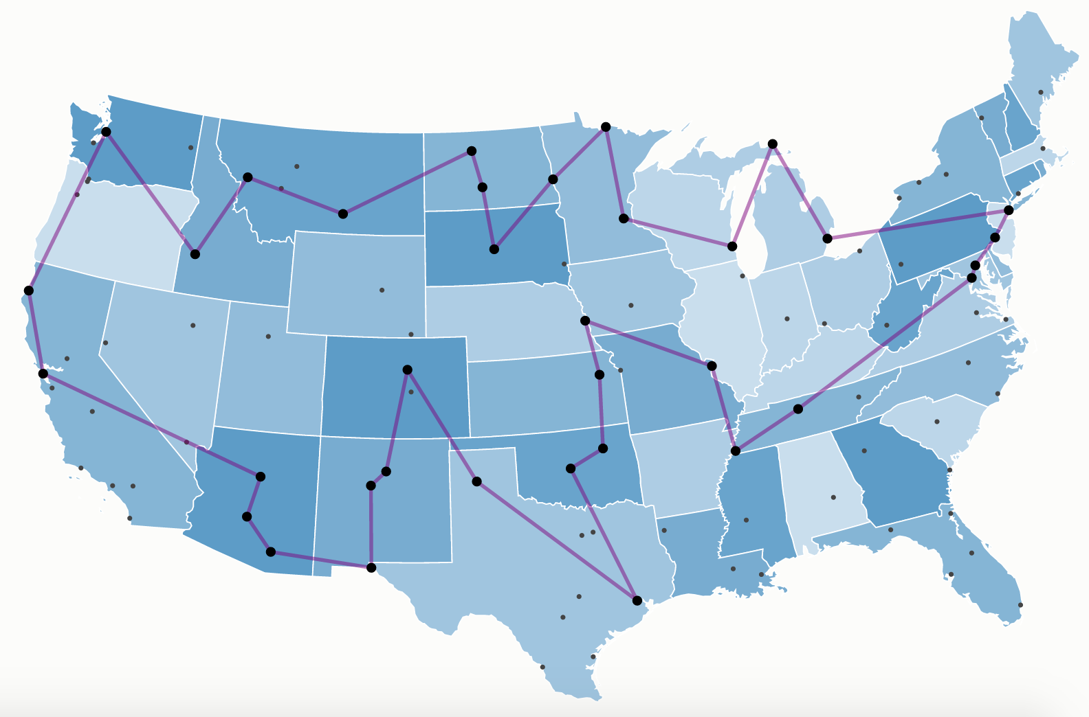
The most well-known publicisation of the problem was recently published by data scientist Dr Randal Olson in 2015, who was challenged by a Discovery news researcher after reading a similar article he published on "Where's Waldo?".
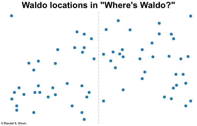
One of his most fascinating observations is the sheer scale of the P vs NP challenge with only 50 destinations:
"With 50 landmarks to put in order, we would have to exhaustively evaluate 3 x 1064 possible routes to find the shortest one. To provide some context: If you started computing this problem on your home computer right now, you’d find the optimal route in about 9.64 x 1052 years."
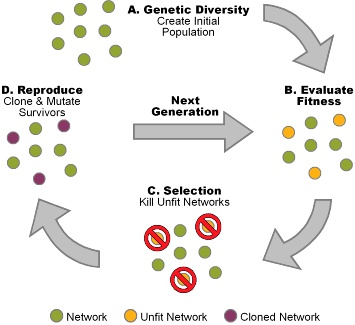
Olson helpfully published his code, which used a genetic algorithm written in Python which iterated over 5000 generations.
For the uninitiated:
"A genetic algorithm is a search heuristic that is inspired by Charles Darwin’s theory of natural evolution. This algorithm reflects the process of natural selection where the fittest individuals are selected for reproduction in order to produce offspring of the next generation. The process of natural selection starts with the selection of fittest individuals from a population. They produce offspring which inherit the characteristics of the parents and will be added to the next generation. If parents have better fitness, their offspring will be better than parents and have a better chance at surviving. This process keeps on iterating and at the end, a generation with the fittest individuals will be found."
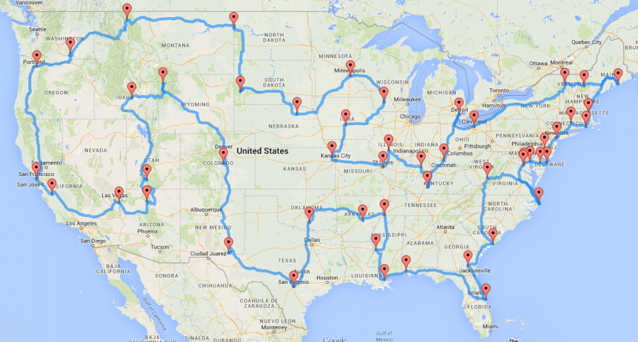
His eventual solution "reached a near-perfect solution that makes a complete trip around the U.S. in only 13,699 miles (22,046 km) of driving."
To his best guess:
"Assuming no traffic, this road trip will take about 224 hours (9.33 days) of driving in total, so it’s truly an epic undertaking that will take at least 2-3 months to complete."
The only question left for any adventurer is: when are we going?