Documents, Fingerprints, Genetics: Storing & Searching Forensic Data

What goes on in the lab and how does it work? The technology behind crime-fighting and detective work we see on TV screens remains strangely opaque, yet much of it is decades old. And fascinating. The unfortunate consequence is innovation around it remains bottlenecked.
Keywords in thousands of documents
The first thing you have in any legal or criminals case is a lot of documentation - in the form of written statements, audio recordings/transcripts, or photographs. You may have tens of thousands, possibly millions.
We need to ask questions, such as:
- Was [keyword] ever mentioned by a suspect?
- How many times has [keyword] been found in these files?
- Who uses [keyword] most on this timeline?
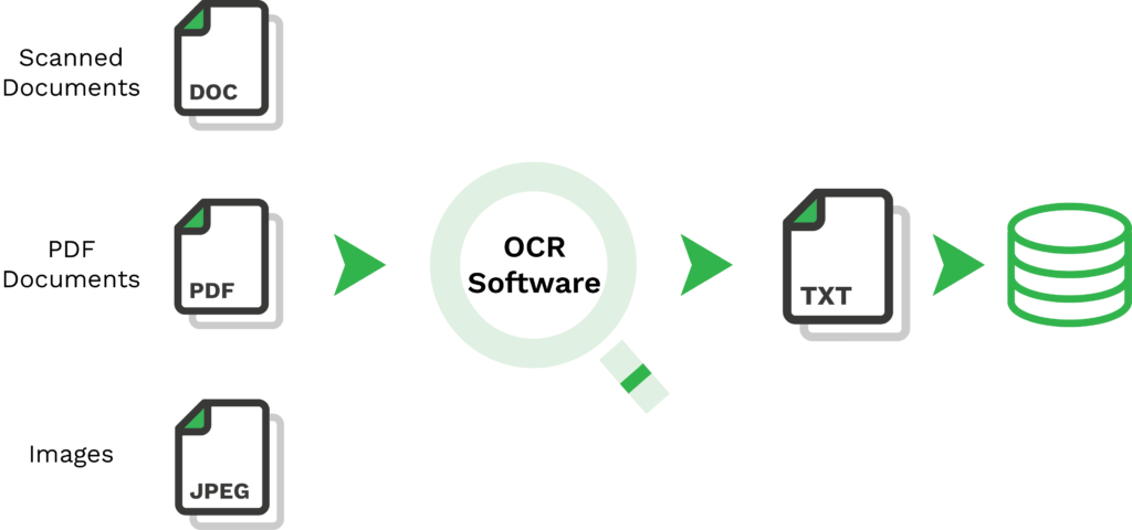
Elasticsearch can index scanned documents (converted to text via OCR), electronic documents, and communications, making them searchable. First, however, we need to get the text out of them.
Text extraction from electronic documents
We won't go fully into how to extract text from electronic documents here. Word documents, PDFs etc are straightforward when it comes to their APIs and content access. Just put together a directory of files, open each file, read what's in it.
Extracting text from an MS Word document, for example: go get github.com/unidoc/unioffice/document :
func main() {

	doc, err := document.Open("path/to/your/document.docx")

	if err != nil {
		log.Fatalf("error opening document: %s", err)
	}

	defer doc.Close()

	for _, para := range doc.Paragraphs() {

		for _, run := range para.Runs() {
			fmt.Print(run.Text())
		}

		fmt.Println()
	}
}
Extracting from a PDF is a little trickier, but still not too tough with the Poppler Tools xPDF library pdftotext tool (https://www.xpdfreader.com/pdftotext-man.html) or Python's PyMuPDF.
Using Go with go get github.com/unidoc/unipdf/v3 :
func main() {

	pdfPath := "path/to/your/document.pdf"

	pdfReader, err := pdf.NewPdfReaderFromFile(pdfPath, nil)

	if err != nil {
		log.Fatalf("Error opening PDF file: %s", err)
	}

	numPages, err := pdfReader.GetNumPages()

	if err != nil {
		log.Fatalf("Error getting number of pages: %s", err)
	}

	for i := 1; i <= numPages; i++ {

		page, err := pdfReader.GetPage(i)

		if err != nil {
			log.Fatalf("Error retrieving page %d: %s", i, err)
		}

		ex, err := extractor.New(page)

		if err != nil {
			log.Fatalf("Error creating extractor: %s", err)
		}

		text, err := ex.ExtractText()

		if err != nil {
			log.Fatalf("Error extracting text: %s", err)
		}

		fmt.Println("Page", i, "Text:", text)
	}
}
A neat trick when extracting PDFs with a reliable structure - screenplays, for example - is to convert them into XML using pdftohtml.
sudo apt-get install poppler-utils

pdftotext path/to/your/document.pdf output.txt

# or

pdftohtml -xml path/to/your/document.pdf output.xml
pdftohtml -stdout path/to/your/document.pdf output.html
The XML output from pdftohtml includes tags that describe the structure and content of the PDF document. For example, you'll see <page> tags for each page in the document, <text> tags for text blocks, along with attributes specifying the position (e.g., top, left), font information, and the actual text content. This structured format can be particularly useful for applications that need to process or analyze the document content in a more detailed manner than plain text extraction would allow. It offers several other options to customize the output, such as -c for complex documents, -hidden to include hidden text, and -nomerge to disable merging of text blocks.
Extracting text from image scans
If we have our JPEG/TIFF images, we can use Hewlett Packard's Tesseract OCR (https://tesseract-ocr.github.io/) to perform Optical Character Recognition on them. This has its limitations, obviously: handwriting isn't simple to understand.
sudo apt-get install tesseract-ocr

mkdir text_output
for image in path/to/your/images/*.jpeg; do
    base=$(basename "$image" .jpeg)
    tesseract "$image" "text_output/$base"
done
This will go over each JPEG image in a directory, converting them to text and saving the output in a separate directory.
The theory is more complex, but it can handle some tricky situations: https://www.researchgate.net/publication/265087843_Optical_character_recognition_applied_on_receipts_printed_in_macedonian_language
Extracting text from photographs
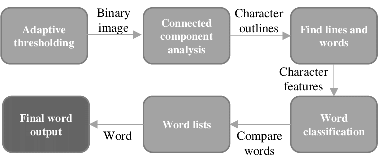
Getting the text out of photos is more difficult. First we need to blur out the noise so the text stands out more clearly.
Preprocessing steps might include resizing, converting to grayscale, increasing contrast, or applying filters to reduce noise. For road signs, which might be captured at an angle, perspective transformation techniques can correct distortions. Applying a thresholding algorithm can help to isolate the text from the background by converting the image to a binary image. Adaptive thresholding techniques can be particularly useful for images with varying lighting conditions.
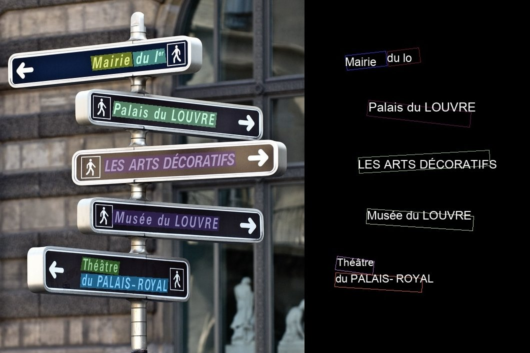
This is where the IBM OpenCV (https://opencv.org/) machine vision library comes in. Combining Python, Tesseract, and OpenCV, we get:
import cv2
import pytesseract

# Load the image
image = cv2.imread('path/to/road_sign.jpg')

# Convert to grayscale
gray = cv2.cvtColor(image, cv2.COLOR_BGR2GRAY)

# Apply adaptive thresholding
thresh = cv2.adaptiveThreshold(gray, 255, cv2.ADAPTIVE_THRESH_GAUSSIAN_C, cv2.THRESH_BINARY, 11, 2)

# OCR with Tesseract
custom_config = r'--oem 3 --psm 6'
text = pytesseract.image_to_string(thresh, config=custom_config)

print(text)
Extracting text from audio recordings
If we want to store the text spoken by people, speech-to-text or Automatic Speech Recognition (ASR), can help us with converting spoken language into written text.
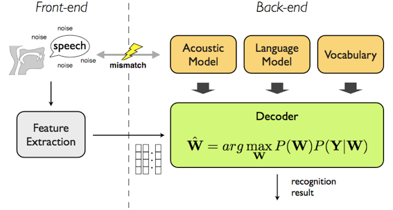
The most popular tools are Carnegie Mellon University's CMU Sphinx (PocketSphinx, https://cmusphinx.github.io/), and Kaldi ASR (https://github.com/kaldi-asr/kaldi). Both require pre-trained models, like more advanced tools such as Mozilla's DeepSpeech.
Once speech is captured, it is broken down into smaller pieces of sound, known as "phonemes," (phonetic pieces) which are the basic units of speech. For example, the word "cat" is broken down into the phonemes "k," "æ," and "t." This is analogous to "tokens" or "n-grams" in normal text. The software looks at the sequence of sounds and tries to match them with patterns it has learned from a vast database of spoken language.
Hidden Markov Models have historically been the backbone of speech recognition systems: https://en.wikipedia.org/wiki/Hidden_Markov_model
The audio must be preprocessed, where it will be noise-reduced to minimize background noise that could interfere with speech recognition; then normalized to adjust the volume for maintaining a consistent level across the recording.
An example using Kaldi:
cd kaldi/egs/your_model_directory

steps/online/nnet2/decode.sh --config conf/decode.config --cmd "run.pl" --nj 1 exp/tri3b/graph data/test exp/tri3b/decode_test
Kaldi models: https://kaldi-asr.org/models.html
An example using PocketSphinx, installed by pip install pocketsphinx:
import os
from pocketsphinx import AudioFile, get_model_path, get_data_path

model_path = get_model_path()
data_path = get_data_path()

config = {
    'verbose': False,
    'audio_file': os.path.join(data_path, 'your_audio_file.wav'),
    'buffer_size': 2048,
    'no_search': False,
    'full_utt': False,
    'hmm': os.path.join(model_path, 'en-us'),
    'lm': os.path.join(model_path, 'en-us.lm.bin'),
    'dict': os.path.join(model_path, 'cmudict-en-us.dict')
}

audio = AudioFile(**config)
for phrase in audio:
    print(phrase)
Acoustic models: https://sourceforge.net/projects/cmusphinx/files/Acoustic and Language Models/
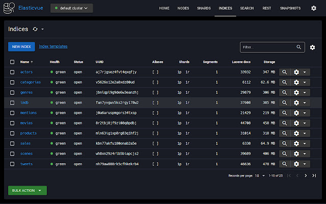
Creating a search engine
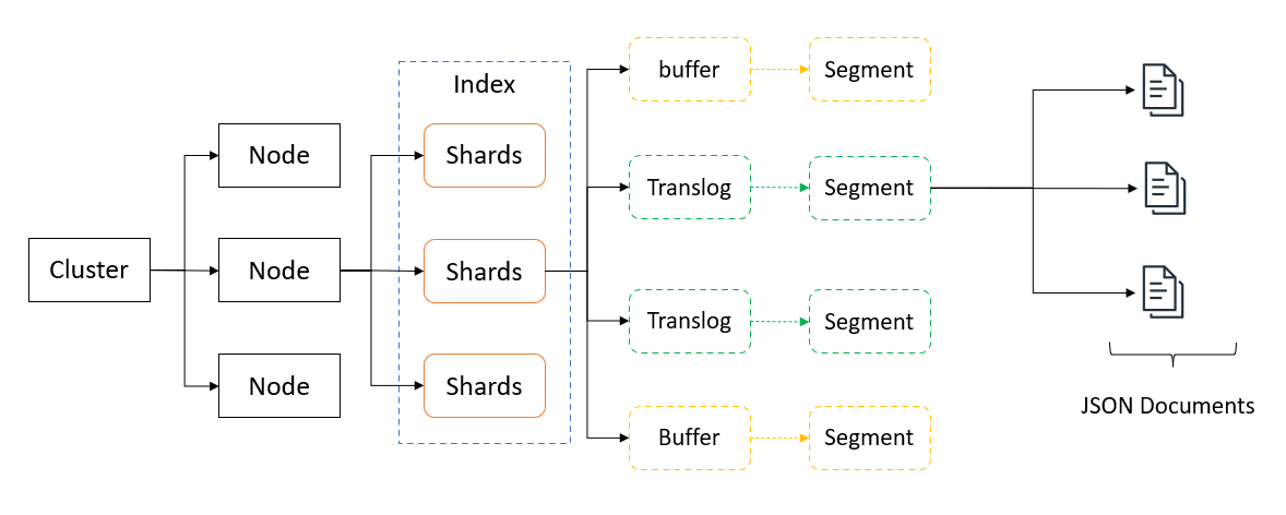
Our Elasticsearch setup is trivial, but building a full search index is not. Particularly with a billion records. The general rule with Elasticsearch is to store documents in the way you would like them to be returned. Ideally, you want the reference to the sentence, paragraph, page; text highlighted; everything scored.
If you index a whole page, you'll have to look through the page of text to find the result. So break it down for storage accordingly. Store by the sentence if possible; paragraph if not; rarely by anything larger.
To create a local instance of Elasticsearch:
docker network create elastic
docker run --name elasticsearch --net elastic -p 9200:9200 -it -m 4GB elasticsearch:8.12.0
We can connect to the REST API on https://localhost:9200 with the username elastic and the password printed into log for the container.
Assuming we set up a single field/column named "content" on an index named "documents", we can feed in the extracted text to Elasticsearch like so:
from elasticsearch import Elasticsearch
import os

es = Elasticsearch()
directory = 'path/to/text_output'

for filename in os.listdir(directory):
    if filename.endswith(".txt"):
        filepath = os.path.join(directory, filename)
        with open(filepath, 'r') as file:
            content = file.read()
        es.index(index="documents", body={"content": content})
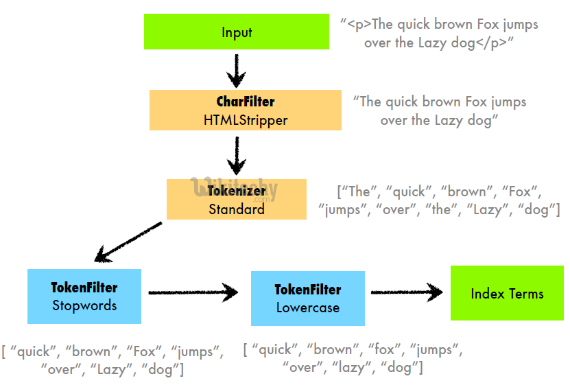
The best choices depend on the nature of the data and the specific needs of the investigation or research. However, some generally useful analyzers and filters within Elasticsearch include:
- Standard Analyzer: Good for general text analysis, breaking text into tokens based on language rules. Useful for a broad range of data types.
- Language-specific Analyzers: Elasticsearch offers built-in analyzers for many languages (e.g., English, Spanish, Russian). These analyzers understand the nuances of the respective language, including stemming, stopwords, and more, making them invaluable for analyzing documents in specific languages.
- Synonym Filter: Helps in finding documents that use different terms to refer to the same concept. For example, in legal research, synonyms can match "homicide" with "murder."
- Stopword Filter: Removes common words that are unlikely to be relevant to searches but can be customized to retain legal or investigation-specific terms that might be considered stopwords in other contexts.
- Edge N-Gram Tokenizer/Filter: Useful for autocomplete features in search applications, helping investigators to quickly find relevant documents by typing only part of a word.
- Custom Analyzers: Creating a custom analyzer by combining tokenizers and filters like lowercase, asciifolding (for handling accents), or pattern_capture (for extracting specific patterns like phone numbers or case numbers) can tailor the search experience to the specific needs of criminal or legal investigations.
Much of the theory here is expanded on in a previous post: https://devilslane.com/a-searchable-multi-language-bible-in-less-than-hour-with-elasticsearch-go/
For which the code is here: https://github.com/devilslane-com/bible-golang-elasticsearch
Building the most accurate search configuration
The logic for a search engine is nuanced, and has to be carefully balanced. It you index too much, you get noise and inaccuracy because of all the false positives. If you go too far, you lose performance. What we want is relevance and accuracy, and that's tricky.
Google's approach - PageRank - thinks about this problem using the citations in academic papers as "votes" or "links back" to the original paper; the more citations a paper has, the more credible and authoritative it is. We only have the text to work with.
However, in general, a strong analyzer configuration for our index "documents" with its single field "content" might look something like this:
PUT /documents
{
  "settings": {
    "analysis": {
      "char_filter": {
        "remove_line_breaks": {
          "type": "pattern_replace",
          "pattern": "\\r\\n|\\r|\\n",
          "replacement": " "
        }
      },
      "filter": {
        "english_stop": {
          "type": "stop",
          "stopwords": "_english_"
        },
        "english_stemmer": {
          "type": "stemmer",
          "language": "english"
        },
        "english_possessive_stemmer": {
          "type": "stemmer",
          "language": "possessive_english"
        },
        "synonym_filter": {
          "type": "synonym",
          "synonyms": [
            "homicide, murder",
            "arson, fire setting",
            "theft, stealing, burglary",
            "assault, attack",
            "vehicle, car, automobile"
            // Add more synonyms relevant to criminal investigation
          ]
        },
        "custom_ngram": {
          "type": "edge_ngram",
          "min_gram": 3,
          "max_gram": 10
        },
        "lowercase_filter": {
          "type": "lowercase"
        },
        "asciifolding_filter": {
          "type": "asciifolding",
          "preserve_original": true
        }
      },
      "analyzer": {
        "criminal_investigation_analyzer": {
          "type": "custom",
          "char_filter": [
            "html_strip",
            "remove_line_breaks"
          ],
          "tokenizer": "standard",
          "filter": [
            "lowercase_filter",
            "english_stop",
            "english_possessive_stemmer",
            "english_stemmer",
            "synonym_filter",
            "asciifolding_filter",
            "custom_ngram"
          ]
        }
      }
    }
  },
  "mappings": {
    "properties": {
      "content": {
        "type": "text",
        "analyzer": "criminal_investigation_analyzer"
      }
    }
  }
}
Character Filters:
html_strip: Removes HTML tags from the text, useful for scanned documents that have been converted to text and might contain HTML artifacts.remove_line_breaks: Converts line breaks to spaces, ensuring that OCR'ed text flows continuously without unnecessary breaks affecting tokenization.
Tokenizer:
standard: Splits text into tokens on word boundaries, suitable for a wide range of languages.
Filters:
lowercase_filter: Converts all tokens to lowercase to ensure case-insensitive matching.english_stop: Removes common English stop words to reduce noise in the text.english_possessive_stemmer: Removes possessive endings from English words ('s) to normalize token forms.english_stemmer: Reduces English words to their stem forms, helping to match different word forms (e.g., "running" and "runs").synonym_filter: Maps synonyms to a common term, enhancing the ability to find relevant documents regardless of the specific terminology used.asciifolding_filter: Converts accents and other diacritics to their ASCII equivalents, improving the matching of accented and unaccented forms.custom_ngram: Generates edge n-grams from each token, aiding in partial word matching and autocomplete functionalities.
This configuration aims to robustly process and index the content of scanned documents, enhancing search capabilities in the context of criminal investigations. It addresses various challenges, including language normalization, synonym handling, and partial match support, making it easier for investigators to find relevant information across a broad dataset.
Indexing and searching fingerprint images
Fingerprinting is old tech. Really old. In 1823 Czech physician Jan Evangelista Purkyně found 9 patterns. Scotland Yard started looking at them in 1840, and the first application of them on contractual documents was performed in 1877, in India, by Sir William James Herschel.
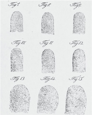
Basic academic theory of minutiae
From Leftipedia, our usual baseline:
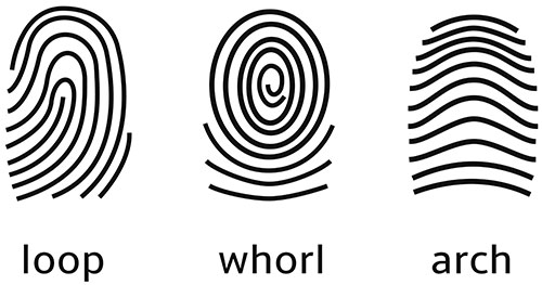
The three basic patterns of fingerprint ridges are the arch, loop, and whorl:
Arch: The ridges enter from one side of the finger, rise in the center forming an arc, and then exit the other side of the finger.
Loop: The ridges enter from one side of a finger, form a curve, and then exit on that same side.
Whorl: Ridges form circularly around a central point on the finger.
Scientists have found that family members often share the same general fingerprint patterns, leading to the belief that these patterns are inherited.
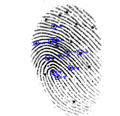
The uniqueness of a fingerprint can be established by the overall pattern of ridges and valleys, or the logical ridge discontinuities known as minutiae. In the 2000s, minutiae features were considered the most discriminating and reliable feature of a fingerprint. Therefore, the recognition of minutiae features became the most common basis for automated fingerprint verification. The most widely used minutiae features used for automated fingerprint verification were the ridge ending and the ridge bifurcation.
Most major algorithms focus on the same theoretical markers:
- Minutiae-Based Matching: The most common approach, focusing on the patterns of ridges and bifurcations (splits) on a fingerprint. Algorithms compare the minutiae points between two fingerprints to find a match.
- Pattern Matching: This involves comparing the overall patterns of ridges and valleys on the fingerprints, including loops, whorls, and arches.
- Ridge Feature-Based Matching: Goes beyond minutiae to include ridge patterns, frequency, and orientation for matching, providing more details for comparison.
- Hybrid Matching: Combines multiple types of features, such as minutiae points, ridge patterns, and skin elasticity, to improve accuracy and robustness against poor quality prints.
Instead of storing the raw fingerprint image, which would require a vast amount of storage space and be inefficient for searching, the system extracts unique features from the fingerprint. These features include these minutiae points (where ridge lines end or fork), ridges, and patterns (like loops, whorls, and arches). Essentially the X/Y vertices within the image.
The extracted features are converted into a digital representation known as a fingerprint template. This template is a compact, encrypted binary file that represents the fingerprint's unique characteristics. The fingerprint template is stored in a database. Each template is associated with the identity of the person to whom the fingerprint belongs.
These templates are somewhat standardised:
ANSI INCITS 378:2009/AM 1:2010[R2015], abbreviated ANSI 378-2009/AM1 or just ANSI 378-2009 or ANSI 378, is a small backwards-compatible update to ANSI 378-2009 published by ANSI in 2010. It is the third version of ANSI's minutia-based fingerprint template format.
ISO/IEC 19794-2:2011/Cor.1:2012, abbreviated ISO 19794-2:2011 or just ISO 19794-2, is a minutia-based fingerprint template format published by ISO in 2011. It is a major redesign of ISO 19794-2:2005 that shares very little with its predecessor. It is incompatible with ANSI 378-2009 even though it shares magic header and version number with it. Smartcard variation is described separately.
https://templates.machinezoo.com/
https://www.iso.org/standard/61610.html
Available biometric analysis software
Fingerprinting software falls into open-source and commercial categories. Commercial providers include:
- NEC Fingerprint Identification Technology: https://www.nec.com/en/global/solutions/biometrics/fingerprint/index.html
- HID Tenprint (Crossmatch): https://www.hidglobal.com/product-mix/tenprint-scanners-dual-finger-scanners
- 3M Cogent (Thales): https://www.cardlogix.com/product-tag/cogent/
- Morpho (IDEMIA): https://na.idemia.com/security/fingerprinting/
- Suprema BioStar: https://www.supremainc.com/en/platform/hybrid-security-platform-biostar-2.asp
- Innovatrics Automated Fingerprint Identification System (AFIS): https://www.innovatrics.com/innovatrics-abis/
The oldest open-source fingerprinting applications were SourceAFIS (https://sourceafis.machinezoo.com/) and OpenAFIS (https://github.com/neilharan/openafis)
SourceAFIS has Java and .Net implementations, e.g. https://sourceafis.machinezoo.com/java
var probe = new FingerprintTemplate(
    new FingerprintImage(
        Files.readAllBytes(Paths.get("probe.jpeg")),
        new FingerprintImageOptions()
            .dpi(500)));
var candidate = new FingerprintTemplate(
    new FingerprintImage(
        Files.readAllBytes(Paths.get("candidate.jpeg")),
        new FingerprintImageOptions()
            .dpi(500)));
double score = new FingerprintMatcher(probe)
    .match(candidate);
boolean matches = score >= 40;
OpenAFIS is fairly impenetrable for juniors, sadly. Its similarity matching is a sight to behold:
#include "OpenAFIS.h"
...
TemplateISO19794_2_2005<uint32_t, Fingerprint> t1(1);
if (!t1.load("./fvc2002/DB1_B/101_1.iso")) {
// Load error;
}
TemplateISO19794_2_2005<uint32_t, Fingerprint> t2(2);
if (!t2.load("./fvc2002/DB1_B/101_2.iso")) {
// Load error;
}
MatchSimilarity match;
uint8_t s {};
match.compute(s, t1.fingerprints()[0], t2.fingerprints()[0]);
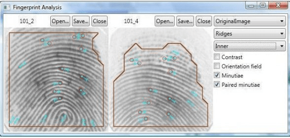
std::cout << "similarity = " << s;Extracting the fingerprint data using NBIS
The best known open-source kit is NBIS (National Institute of Standards and Technology Biometric Image Software, https://www.nist.gov/services-resources/software/nist-biometric-image-software-nbis), which includes its Bozorth3 algorithm.
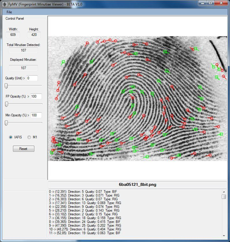
NBIS has everything baked in. Pulling out the data from your JPG, BMP, or TIFF image file is as simple as running the mindtct tool:
mindtct -m1 my_fingerprint.bmp my_fingerprint_output
"mindtct" stands for MINutiae DecTeCTion (MINDTCT) and its workflow logic is well-documented:
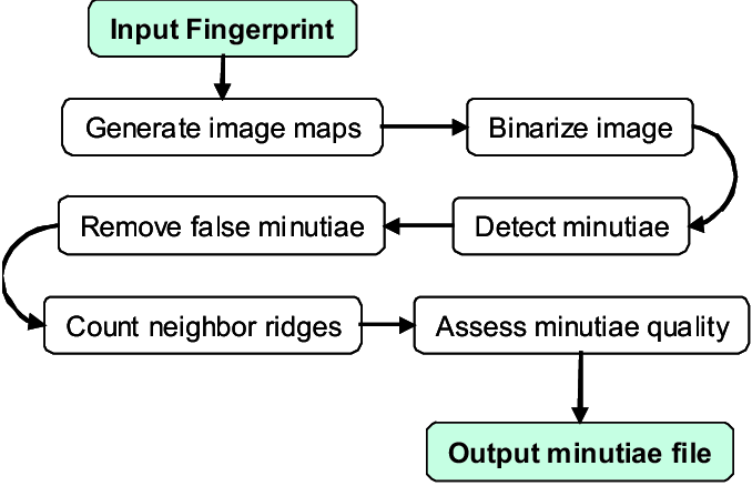
Source: https://github.com/lessandro/nbis
After running mindtct, you'll have several binary output files, including:
my_fingerprint_output.min: The binary minutiae file, which contains the extracted minutiae points.my_fingerprint_output.xytm: A human-readable text file listing the minutiae coordinates, type (ridge ending or bifurcation), and direction.
The .min file format is specific to NBIS and stores minutiae and other data in a binary format that's optimized for processing and comparison by NBIS tools. It's not meant to be human-readable and requires specific software (like NBIS itself) to interpret.
The .xytm file, on the other hand, is a text representation of the minutiae points found in a fingerprint image. It typically contains lines of data where each line represents a single minutia, with each line formatted something like:
X-coordinate Y-coordinate Type Direction
150 248 E 65- X-coordinate and Y-coordinate are the pixel coordinates of the minutia on the fingerprint image.
- Type indicates whether the minutia is a ridge ending (often denoted by "E") or a bifurcation (denoted by "B").
- Direction is the angle (in degrees or another unit) indicating the orientation of the ridge on which the minutia is found.
The Bozorth3 algorithm is then used for searching. It operates by comparing pairs of minutiae between two fingerprints, and in general, it:
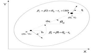
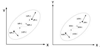
- Uses minutiae points extracted from fingerprints, including their location, orientation, and type.
- Analyzes pairs of minutiae between two fingerprints, assessing spatial and directional relationships.
- Groups similar minutiae pairs into sets based on their spatial and directional congruence.
- Calculates a match score from the matching sets, where higher scores indicate a better match.
- Determines if fingerprints match based on whether the score crosses a predefined threshold.
More on the algo: https://github.com/lessandro/nbis/blob/master/bozorth3/src/lib/bozorth3/bozorth3.c
Storing and searching binary data with PostgreSQL
Fingerprint "templates" are stored as binary blobs or byte arrays, but you can't search them directly with PostgreSQL or any other RDBMS server engines as you would using normal SQL.
So once we have extracted the geometric "template", we'd add it to a database, for example, like so:
CREATE TABLE fingerprint_templates (
    id SERIAL PRIMARY KEY,
    template BYTEA NOT NULL,
    pattern_type VARCHAR(50),
    created_at TIMESTAMP WITH TIME ZONE DEFAULT CURRENT_TIMESTAMP
);
And we'd add them in the usual way:
INSERT INTO fingerprint_templates (template, pattern_type)
VALUES (<binary_template>, 'whorl');
When using the aforementioned NBIS data, we'd also use binary fields in Postgres, but combine them with raw text and metadata to narrow things down.
CREATE TABLE fingerprint_data (
    id SERIAL PRIMARY KEY,
    minutiae_data BYTEA,
    minutiae_text_data BYTEA,
    minutiae_count INT, -- Number of minutiae points, useful for quick filtering
    average_minutiae_quality FLOAT, -- Optional, for filtering by quality
);
And store them programmatically, directly into the blob columns.
import psycopg2

# Connect to your PostgreSQL database
conn = psycopg2.connect("dbname=your_db user=your_user password=your_password")
cur = conn.cursor()

# Read the binary data from the .min file
with open('my_fingerprint_output.min', 'rb') as file:
    minutiae_data = file.read()

# Read the binary data from the .xytm file
with open('my_fingerprint_output.xytm', 'rb') as file:
    minutiae_text_data = file.read()

# Insert the data into the database
cur.execute(
    "INSERT INTO fingerprint_data (minutiae_data, minutiae_text_data) VALUES (%s, %s)",
    (psycopg2.Binary(minutiae_data), psycopg2.Binary(minutiae_text_data))
)

# Commit the transaction and close
conn.commit()
cur.close()
conn.close()
What we do need to know is how many minutiae points have been captured.
An interesting sidebar is pgAFIS (Automated Fingerprint Identification System support for PostgreSQL): https://github.com/hjort/pgafis. The plugin attempts to provide full search support on the database side, with custom column data types.
Author Rodrigo Hjort explains:
"pgm" stores fingerprints raw images (PGM)
"wsq" stores fingerprints images in a compressed form (WSQ)
"mdt" stores fingerprints templates in XYTQ type in a binary format (MDT)
"xyt" stores fingerprints minutiae data in textual form
The data type used in these columns is "bytea" (an array of bytes), similar to BLOB in other DBMSs. PGM and WSQ formats are open and well-known in the market.
https://agajorte.blogspot.com/2015/09/pgafis-biometric-elephant.html
It's cool, even if it's not the most efficient thing in the world.
UPDATE fingerprints SET wsq = cwsq(pgm, 2.25, 300, 300, 8, null) WHERE wsq IS NULL;
UPDATE fingerprints SET mdt = mindt(wsq, true) WHERE mdt IS NULL;

SELECT (bz_match(a.mdt, b.mdt) >= 20) AS match
FROM fingerprints a, fingerprints b
WHERE a.id = '101_1' AND b.id = '101_6';

SELECT a.id AS probe, b.id AS sample,
  bz_match(a.mdt, b.mdt) AS score
FROM fingerprints a, fingerprints b
WHERE a.id = '101_1' AND b.id != a.id
  AND bz_match(a.mdt, b.mdt) >= 23
LIMIT 3;
If we can get a Postgres implement for SMILES data in chemistry (https://www.rdkit.org/docs/Cartridge.html), how hard can it be to add one for AFIS?
Bonus: open source hardware
An honourable mention is RaspiReader, developed at Michigan State University as a fingerprint reader attached to a Raspberry Pi.
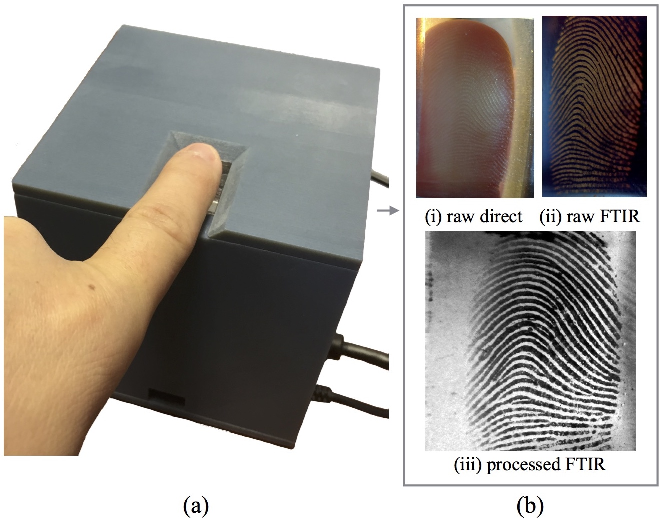
The Camera Adaptor uses the RPi.GPIO Python package. The RaspiReader performs image processing, and its spoof detection takes image colour and 3D friction ridge patterns into account. The detection algorithm extracts colour local binary patterns.
https://www.raspberrypi.com/news/raspireader-fingerprint-scanner-2/
RaspiReader: Open Source Fingerprint Reader
Joshua J. Engelsma, Kai Cao, and Anil K. Jain, Life Fellow, IEEE
https://biometrics.cse.msu.edu/Publications/Fingerprint/EngelsmaKaiJain_RaspiReaderOpenSourceFingerprintReader_TPAMI2018.pdf
Genetic marker identification and similarity
Let's face it, the genetics graphs on TV dramas look cool. But how does the generic profiling actually work, once you extract samples?
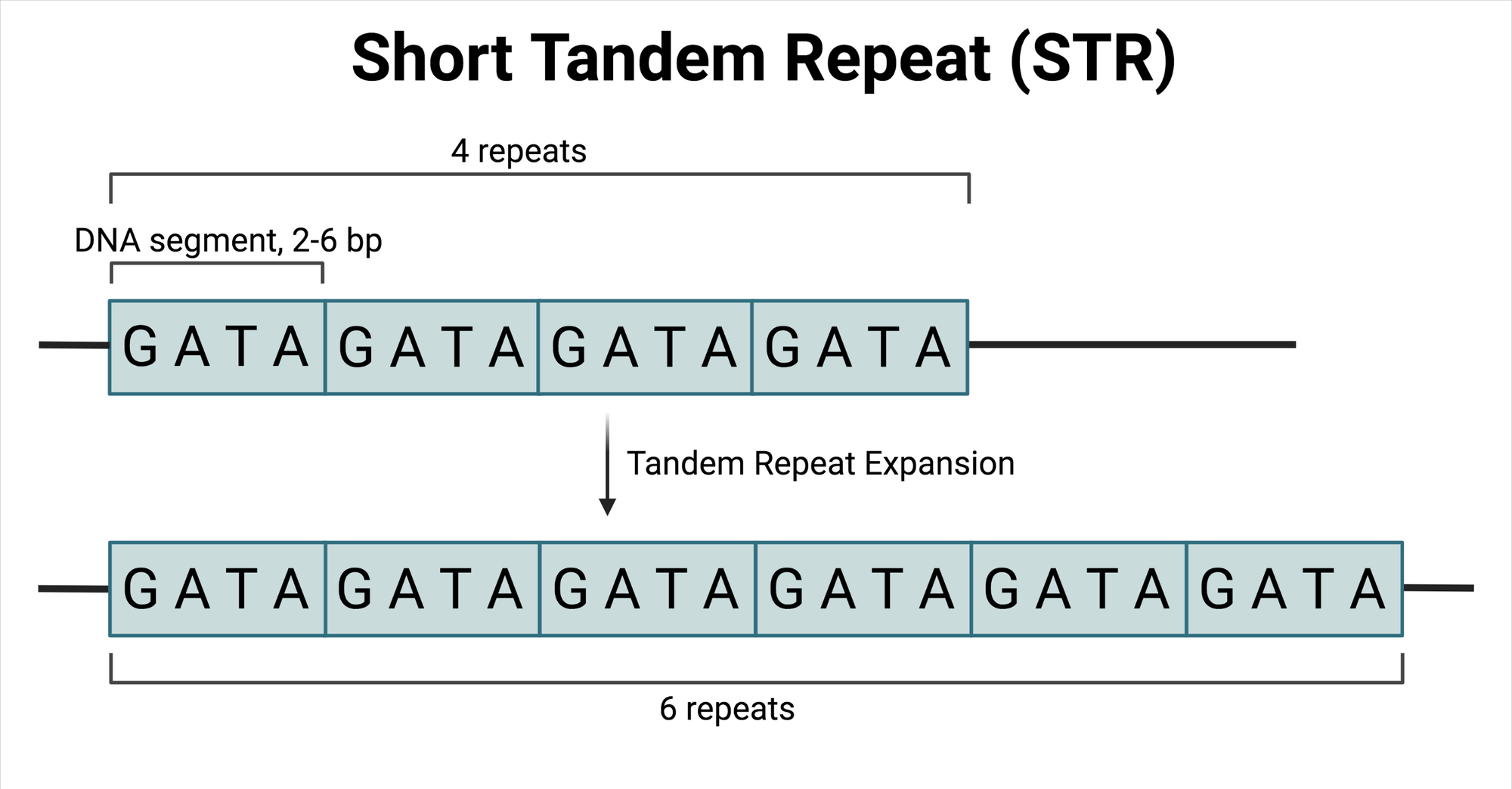
A DNA profile is a recording of Short Tandem Repeat (STR) markers, not your whole genome. These are "shortcut" regions of your DNA where certain patterns of nucleotides are repeated. They are information on the specific STR loci (locations on the chromosome), the number of repeats at each locus, and an identification number for the sample.
Matching STR profiles involves comparing these repeat numbers between samples. A match may be declared if the profiles are identical or if there's a high degree of similarity across the loci.
Understanding Short Tandem Repeats (STRs)
Short Tandem Repeats (STRs) are critical markers used in genetic profiling, especially in forensic science, due to their high variability among individuals.
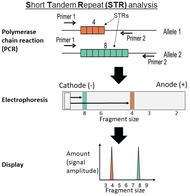
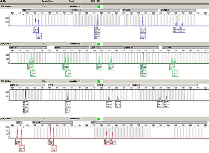
PCR (Polymerase Chain Reaction) is used to amplify the STR regions. Capillary electrophoresis is then employed to separate the amplified STR regions and detect them with a laser and fluorescent dyes. Finally, software analyzes the lengths of the amplified STR regions, determining the number of repeats at each locus.
The resulting data for an individual at a given STR locus is represented as two whole numbers (for autosomal STRs), corresponding to the number of repeats inherited from each parent, e.g., "12, 14" at the D8S1179 locus.
(A locus is the specific physical location of a gene or other DNA sequence on a chromosome, like a "genetic street address").
An example STR profile for an individual might be:
- D8S1179: 13, 14
- D21S11: 28, 30
- D18S51: 17, 19
- TH01: 6, 9
- FGA: 22, 25
Another individual's STR profile might be:
- D8S1179: 13, 14 <— same
- D21S11: 29, 30 <— one point away
- D18S51: 17, 20 <— one point away
- TH01: 6, 9 <— same
- FGA: 22, 24 <— one point away
Comparing these two profiles, one can see they are very similar, indicating a potential familial relationship if not an exact match. Which means we don't need any kind of algorithm, we simply need the absolute diff. We can plot them as spikes or bars on a graph.
The core genetic markers
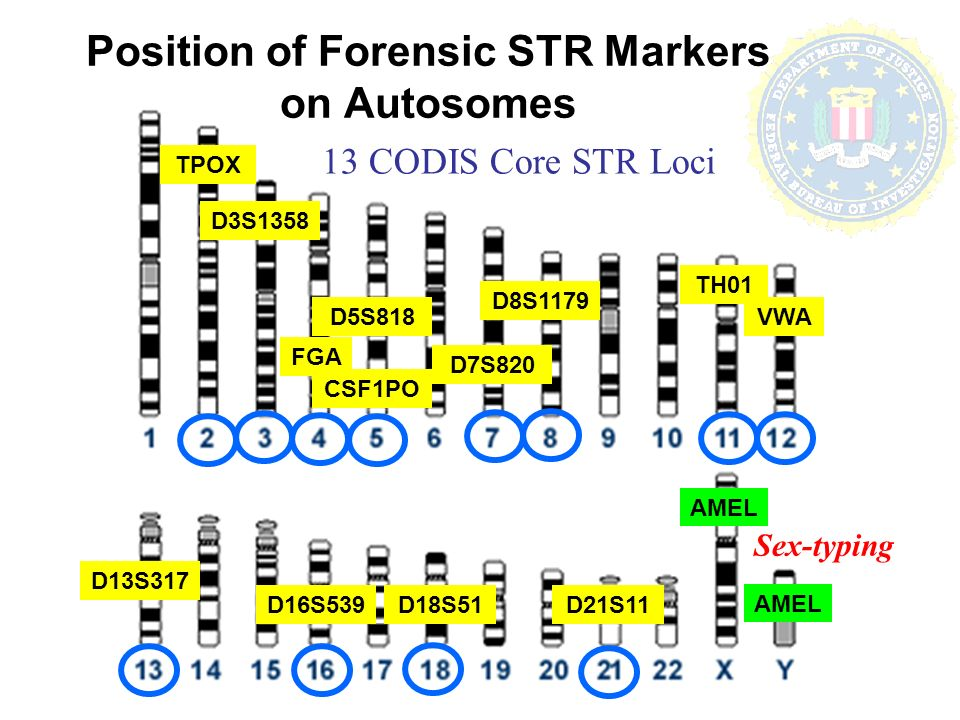
The 20 core STR loci markers used in the Combined DNA Index System (CODIS), established by the FBI, are selected for their high variability among individuals, making them highly effective for forensic identification.
Each marker does not identify specific traits or characteristics but rather serves as a point of comparison for individual genetic profiles.
- D3S1358: Identifies variations in the DNA sequence at the D3S1358 locus on chromosome 3.
- vWA: Targets variability in the von Willebrand factor gene on chromosome 12, important for blood clotting.
- D16S539: Focuses on sequence variations at the D16S539 locus on chromosome 16.
- CSF1PO: Identifies variations in the colony-stimulating factor 1 receptor gene on chromosome 5.
- TPOX: Targets variability in the thyroid peroxidase gene on chromosome 2, involved in thyroid hormone synthesis.
- Y-STRs: Identifies male-specific variations in the Y chromosome, useful for tracing paternal lineage.
- Amelogenin: Determines gender by identifying differences in the X and Y chromosome versions of the amelogenin gene, involved in tooth enamel formation.
- D8S1179: Focuses on sequence variations at the D8S1179 locus on chromosome 8.
- D21S11: Identifies variations at the D21S11 locus on chromosome 21.
- D18S51: Targets variations at the D18S51 locus on chromosome 18.
- D2S441: Identifies sequence variations at the D2S441 locus on chromosome 2.
- D19S433: Focuses on variability at the D19S433 locus on chromosome 19.
- TH01: Targets variations in the tyrosine hydroxylase gene on chromosome 11, which is involved in neurotransmitter synthesis.
- FGA: Identifies variability in the fibrinogen alpha chain gene on chromosome 4, important for blood clotting.
- D22S1045: Focuses on variations at the D22S1045 locus on chromosome 22.
- D5S818: Identifies variations at the D5S818 locus on chromosome 5.
- D13S317: Targets sequence variations at the D13S317 locus on chromosome 13.
- D7S820: Identifies variations at the D7S820 locus on chromosome 7.
- D10S1248: Focuses on variability at the D10S1248 locus on chromosome 10.
- D1S1656: Identifies variations at the D1S1656 locus on chromosome 1.
Each of these markers is chosen for its polymorphic nature, allowing forensic scientists to generate a unique DNA profile for an individual based on the specific alleles (versions of a gene) present at these loci.
Genetic analysis software
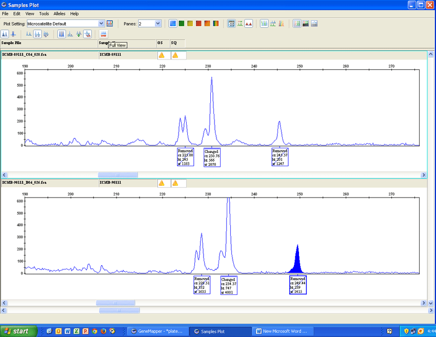
There are two main pieces of gene software used in the lab. The first, ThermoFisher's GeneMapper (https://www.thermofisher.com/order/catalog/product/4475073), is widely used everywhere.
The second, STRmix (https://www.strmix.com/), is specific to the forensic world and used more than the open-source web app cousin, STRait Razor, (https://github.com/ExpectationsManaged/STRaitRazorOnline).
In general, open source software is limited when it comes to forensics, but LRmix Studio (https://github.com/smartrank/lrmixstudio) and Verogen ForenSeq Universal Analysis (https://verogen.com/products/universal-analysis-software/) come closest.
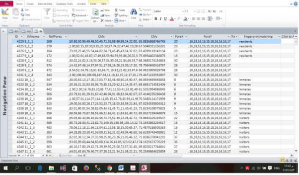
Storing genetic data in a database
Thankfully this is trivial, as all the work is done by the lab machines in extracting them and getting the numbers. And there are a fixed number of markers, meaning it's easy to store them as columns.
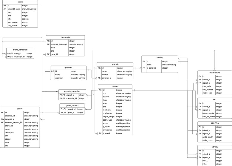
Schema from "WebSTR: A Population-wide Database of Short Tandem Repeat Variation in Humans"
https://www.sciencedirect.com/science/article/pii/S0022283623003716
Using a heavily-indexed table, we can simply use parallel INT fields. Note: these values come in pairs of alleles, it's not this simple. Each reading is two values, so we'd need a JSONB field or double the amount of columns.
CREATE TABLE str_profiles (
    id SERIAL PRIMARY KEY,
    user_id INT,
    D3S1358 INT,
    vWA INT,
    D16S539 INT,
    CSF1PO INT,
    TPOX INT,
    Y_IND INT, -- Indicator for the presence of Y-STRs, if applicable
    AMELOGENIN INT, -- For sex determination
    D8S1179 INT,
    D21S11 INT,
    D18S51 INT,
    D2S441 INT,
    D19S433 INT,
    TH01 INT,
    FGA INT,
    D22S1045 INT,
    D5S818 INT,
    D13S317 INT,
    D7S820 INT,
    D10S1248 INT,
    D1S1656 INT,
    PENTA_D INT, -- Additional markers beyond the core 20 CODIS markers
    PENTA_E INT,
    SE33 INT,
    D6S1043 INT,
    D12S391 INT,
    D2S1338 INT,
    created_at TIMESTAMP WITHOUT TIME ZONE DEFAULT CURRENT_TIMESTAMP,
    updated_at TIMESTAMP WITHOUT TIME ZONE DEFAULT CURRENT_TIMESTAMP,
    FOREIGN KEY (user_id) REFERENCES users (id)
);

CREATE INDEX idx_str_profiles_user_id ON str_profiles(user_id);
CREATE INDEX idx_str_profiles_D3S1358 ON str_profiles(D3S1358);
CREATE INDEX idx_str_profiles_vWA ON str_profiles(vWA);
/* etc etc */
Queries could be as simple as:
SELECT * FROM str_profiles
WHERE D3S1358 = 15 AND vWA = 17 AND D16S539 = 12
If we have a set of markers, like for the example above, we can calculate the DIFF easily. A match means zero (0) difference.
Given these scores:
D8S1179: 13, 14
D21S11: 28, 30
D18S51: 17, 19
TH01: 6, 9
FGA: 22, 25
SELECT record_id,
       individual_id,
       ABS(D8S1179 - 13) AS D8S1179_diff,
       ABS(D21S11 - 28) AS D21S11_diff,
       ABS(D18S51 - 17) AS D18S51_diff,
       ABS(TH01 - 6) AS TH01_diff,
       ABS(FGA - 22) AS FGA_diff,
       (ABS(D8S1179 - 13) + ABS(D21S11 - 28) + ABS(D18S51 - 17) + ABS(TH01 - 6) + ABS(FGA - 22)) AS total_diff
FROM str_profiles
ORDER BY total_diff ASC;
(Since each marker can have two values (alleles), and the database structure stores only a single integer per marker (which might represent one allele, the most common allele, or a summarization of the data), this is simplified.)
If we don't want to use a Postgres ARRAY field/column, perhaps we have these as INT columns:
D8S1179_A
D8S1179_B
D21S11_A
D21S11_B
D18S51_A
D18S51_B
TH01_A
TH01_B
FGA_A
FGA_B
Here, of course, our query needs to become more annoying. There are other ways, but we're explaining verbosely how it can become complicated, quickly.
SELECT id, user_id,
    (D8S1179_A = 13 OR D8S1179_A = 14 OR D8S1179_B = 13 OR D8S1179_B = 14) +
    (D21S11_A = 28 OR D21S11_A = 30 OR D21S11_B = 28 OR D21S11_B = 30) +
    (D18S51_A = 17 OR D18S51_A = 19 OR D18S51_B = 17 OR D18S51_B = 19) +
    (TH01_A = 6 OR TH01_A = 9 OR TH01_B = 6 OR TH01_B = 9) +
    (FGA_A = 22 OR FGA_A = 25 OR FGA_B = 22 OR FGA_B = 25) AS similarity_score
FROM str_profiles
WHERE D8S1179_A IN (13, 14) OR D8S1179_B IN (13, 14)
   OR D21S11_A IN (28, 30) OR D21S11_B IN (28, 30)
   OR D18S51_A IN (17, 19) OR D18S51_B IN (17, 19)
   OR TH01_A IN (6, 9) OR TH01_B IN (6, 9)
   OR FGA_A IN (22, 25) OR FGA_B IN (22, 25)
ORDER BY similarity_score DESC;
Similarity matching through distance
We can get a bit wider and cleverer on this by looking at the numerical graph distances between numbers and matches.
SELECT
  id, -- Assuming there's an identifier column for each record
  (D3S1358 - example_D3S1358)^2 AS D3S1358_diff,
  (vWA - example_vWA)^2 AS vWA_diff,
  (D16S539 - example_D16S539)^2 AS D16S539_diff,
  -- Include similar calculations for all STR markers
  ((D3S1358 - example_D3S1358)^2 +
   (vWA - example_vWA)^2 +
   (D16S539 - example_D16S539)^2 +
   -- Add all squared differences
  ) AS total_similarity_score
FROM str_data
ORDER BY total_similarity_score ASC
LIMIT 100;
We could also use Approximate Nearest Neighbor (ANN) (e.g., Locality-Sensitive Hashing, KD-trees for lower-dimensional data) to quickly find the most similar profiles without needing to compare against every single record.
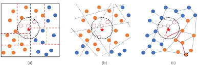
ANN is a technique used to efficiently find points in a space that are close to a given query point, without necessarily performing an exhaustive search.
The pg_trgm module for PostgreSQL (https://www.postgresql.org/docs/current/pgtrgm.html) supports similarity searches on text data using trigram matching. While it's primarily designed for text, creative use or adaptation for numerical data represented as strings might be possible for low-dimensional data.
-- Install the extension
CREATE EXTENSION pg_trgm;

-- Use the % operator for similarity comparison
SELECT * FROM str_profiles WHERE D18S51 % 17;
We could also use:
- Faiss (Facebook AI Similarity Search): a library for efficient similarity search and clustering of dense vectors. It's particularly well-suited for high-dimensional vectors. (More: https://engineering.fb.com/2017/03/29/data-infrastructure/faiss-a-library-for-efficient-similarity-search/)
- Annoy (Spotify: Approximate Nearest Neighbors Oh Yeah): a C++ library with Python bindings for searching in spaces with hundreds of dimensions. It's used for music recommendation algorithms. (More: https://github.com/spotify/annoy)
- HNSW (Hierarchical Navigable Small World): In several libraries, known for its efficiency in high-dimensional nearest neighbor search. (More: https://www.pinecone.io/learn/series/faiss/hnsw/)
For more on ANN: https://towardsdatascience.com/comprehensive-guide-to-approximate-nearest-neighbors-algorithms-8b94f057d6b6
If we were feeling really fancy, we'd use Euclidean Distance or Hamming Distance. The former is more suitable for numerical and continuous data, while the latter is is used for categorical data.

The Euclidean distance between two points in Euclidean space is the length of a line segment between the two points. It can be calculated from the Cartesian coordinates of the points using the Pythagorean theorem. In the context of STR data, each marker (or column) can be considered a dimension in Euclidean space, and the count of repeats for each marker represents a point in that space.
So you're doing geography and geometry, basically.
d(p, q) = sqrt((q1 - p1)^2 + (q2 - p2)^2 + ... + (qn - pn)^2)
Where:
- d(p, q) is the Euclidean distance between two points p and q.
- sqrt represents the square root function.
- (qi - pi) represents the difference between the ith coordinate of point q and the ith coordinate of point p.
- ^2 indicates squaring the difference of each corresponding coordinate.
- The summation is over all the coordinates from 1 to n of the points in the space.
import pandas as pd
from scipy.spatial import distance

# Assuming df is your DataFrame and example_record is a Series or list with the same columns as df
distances = df.apply(lambda row: distance.euclidean(row, example_record), axis=1)

# Add the distances to the DataFrame
df['similarity_score'] = distances

# Sort the DataFrame by the similarity score
sorted_df = df.sort_values(by='similarity_score')
The Euclidean formula is found in almost every programming language. The following use p and q as arrays or lists of coordinates in an n-dimensional space. Each function calculates the sum of the squares of differences between corresponding coordinates of p and q, and then returns the square root of that sum.
Everyone hates maths.
In Go:
func euclidean_distance (p, q []float64) float64 {
    var sum float64

    for i := range p {
        diff := q[i] - p[i]
        sum += diff * diff
    }

    return math.Sqrt(sum)
}
In PHP:
function euclidean_distance (array $p, array $q): float {
    $sum = 0.0;

    for ($i = 0; $i < count($p); $i++)
    {
        $sum += pow($q[$i] - $p[$i], 2);
    }

    return sqrt($sum);
}
And in Python:
def euclidean_distance (p, q):
    return math.sqrt(sum((px - qx) ** 2 for px, qx in zip(p, q)))
A Quick Word On AI
No human can search a library of millions of files mentally. And AI may be useful, but it's not deployable at this point with that kind of private data (yet). It's getting there, but it needs resources. Some can run on laptops, but it's not there so far.
Twitter's "Grok" is trained on the bullshit streamed on Twitter; Facebook/Meta's open source LaMDA (Language Model for Dialogue Applications) is trained on the Boomer-speak from people's profiles. The rest are commercial or community-driven, requiring a lot of tech know-how to implement.
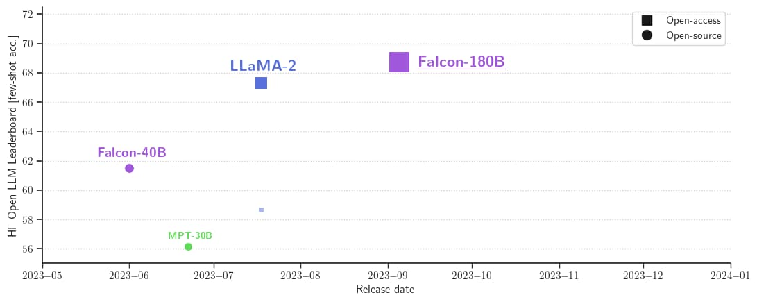
If you're going to start, think about Falcon 180B. It's called that because it's trained with 180 billion parameters, and is just below GPT-4 in ability/performance.
The top open-source large language models (LLMs) are:
- LLaMA 2 (Facebook/Meta): https://llama.meta.com/llama2/
- BLOOM (community): https://huggingface.co/bigscience/bloom
- Falcon 180B (TII/UAE): https://falconllm.tii.ae/falcon-models.html
- GPT-NeoX (EleutherAI): https://huggingface.co/docs/transformers/model_doc/gpt_neox
More: https://github.com/eugeneyan/open-llms
When it comes to most AI, models are developed from the same repository. It is known as "The Pile".
The Pile is a 825 GiB diverse, open source language modelling data set that consists of 22 smaller, high-quality datasets combined together.
To score well on Pile BPB (bits per byte), a model must be able to understand many disparate domains including books, github repositories, webpages, chat logs, and medical, physics, math, computer science, and philosophy papers. Pile BPB is a measure of world knowledge and reasoning ability in these domains, making it a robust benchmark of general, cross-domain text modeling ability for large language models.
https://pile.eleuther.ai/